4. Use of the R DADA2 package to process the 16S rRNA gene sequence reads
Step 1. First we need to create a working directory and download a set of demo Illumina 16S rRNA sequences
#create a directory to work in, so everything is contained in this folder
dir.create("resispart")
#set the working directory to resispart
setwd("resispart")
#double check the currrent working directory is resispart
getwd()
You should see something like this:

Next, do this to download and extract a set of demo files:
#download from an FTP site
download.file("https://github.com/tsute/resispart/releases/download/demo_data/RESISPART_Bioinformatics_Workshop_Demo.zip","demo.zip")

## then unzip it, exdir tells R to just extract to the current working directory "."
unzip("demo.zip",exdir=".")

#list the content of the unzipped files
list.files()
The file size is 1.1Gb so it may take some time to download, depending on the Internet connection speed.

|
If the above link doesn't work try one of these alternative download links: Forsyth Bioinformatics Download Link Google Drive One Drive Dropbox Click on one of the above links and follow the direction to download the file RESISPART_Bioinformatics_Workshop_Demo.zip Find the file on your computer, double-click to unzip it and then move the entire content to the "resispart" working directory. |
Step 2. Find the sequence data
path <- "fastq"
#list.files(path)
fnFs <- sort(list.files(path, pattern="_R1.fastq", full.names = TRUE)) # store forward (R1) sequence files in this object
fnRs <- sort(list.files(path, pattern="_R2.fastq", full.names = TRUE)) # store reverse (R2) sequence files in this object
sample.names <- sapply(strsplit(basename(fnFs), "_"), `[`, 1)

# type the object name to see what sample names we have
sample.names
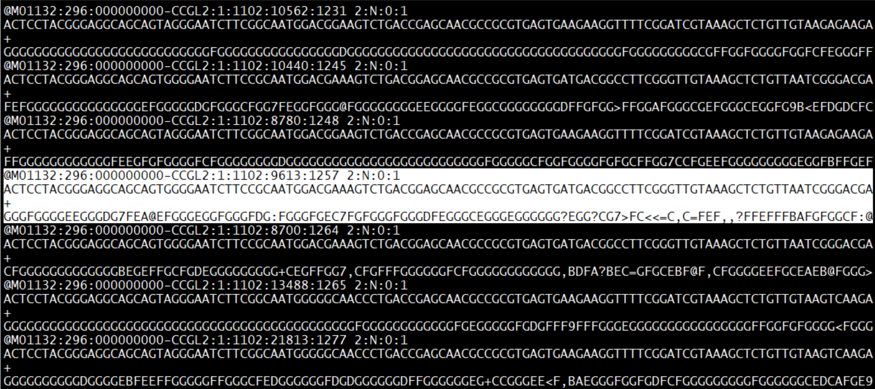
In this workshop we have all together 3,383,251 x 2 sequences in 12 samples (each sample has two files R1 and R2). These are called pair-end reads. The Illumina sequencer can sequence both ends of a DNA amplicon at the same time, expanding the sequence length and span. If the two reads overlap enough we can also merge them together into a single sequence from each pair of the reads. We will process them separately first for quality filtering and later merge them together for downstream analysis.
Step 3. Quality plots
Make a plot for the read pairs (R1 and R2) of the first sample:
plotQualityProfile(c(fnFs[1],fnRs[1]))
Quality plot output:
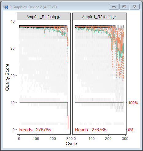
| In gray-scale is a heat map of the frequency of each quality score at each base position. The median quality score at each position is shown by the green line, and the quartiles of the quality score distribution by the orange lines. The red line shows the scaled proportion of reads that extend to at least that position |
Now we make a loop to plot all the read pairs in a single shot:
dir.create("quality_plots", showWarnings = F)

quality_plots=list()
for (i in 1:length(fnRs)) {
quality_plots[[i]]=plotQualityProfile(c(fnFs[i],fnRs[i]))
}
quality_plots_all=ggarrange(plotlist=quality_plots,ncol=1,nrow=length(fnRs))

pdf("quality_plots/quality_plots_all.pdf", width=10, height=3*length(fnRs))
quality_plots_all
dev.off()
You will see some warnings but we can safely ignore them:
This will generate a long PDF file with quality plots for all 12 samples. Go to windows desktop folder “resispart” and the PDF plot is called “quality_plots_all.pdf” in the “quality_plots” folder.
Open the pdf file you will see 12 pairs of quality plots in one pdf file:

The purpose of examining these quality plots is to help us pick a trimming length for the reads. Usually the sequence quality degrades more rapidly toward the end of the read, this is especially so for R2.
Step 4. Filter and trimm sequences
Based on the above sequence plots, we observe that quality score starts to drop rapidly after base 280 for R1 and 220 for R2 so next we will trim the bases off the reads after these two positions:
dir.create("filtered", showWarnings = FALSE)
filtFs <- file.path("filtered", paste0(sample.names, "_F_filt.fastq.gz"))
filtRs <- file.path("filtered", paste0(sample.names, "_R_filt.fastq.gz"))
reads.filtered.start=Sys.time()
reads.filtered <- filterAndTrim(fnFs, filtFs, fnRs, filtRs, truncLen=c(280,220),maxN=0, maxEE=c(2,2), truncQ=2, rm.phix=TRUE,compress=TRUE, multithread=TRUE)
reads.filtered.finished=Sys.time()
| This may take a while depending on your computer's speed. If it is taking too long, we can cancel the "filterAndTrim" command by pressing the Escape key and then the Enter to to cancel the filtering process. We will used a pre-filtered result in the "filtered_backup" folder. Go to Windows explorer and rename this folder to just "filtered" so we can continue to the next step. |
Step 5. Learn sequence error rates to build error models for denoise purpose
The next step is the first phase of the DADA2 amplicon denoising procedure. DADA2 is the second version of the DADA (The Divisive Amplicon Denoising Algorithm)(Rosen et al, 2012). DADA was developed to model the 454-sequenced amplicon data, whereas DADA2 was designed specifically for the Illumina sequence reads (Callahan et al, 2016). In this step we use the quality-filtred reads for building the error models required by the DADA2 denoising algorithm.
dir.create("err_plots", showWarnings = FALSE)

#learnErrors.start=Sys.time()
errF <- learnErrors(filtFs, multithread=TRUE)
errR <- learnErrors(filtRs, multithread=TRUE)
#learnErrors.finished=Sys.time()

plotErrors(errF, nominalQ=TRUE)

pdf("err_plots/errF.pdf")
plotErrors(errF, nominalQ=TRUE)
dev.off()

plotErrors(errR, nominalQ=TRUE)

pdf("err_plots/errR.pdf")
plotErrors(errR, nominalQ=TRUE)
dev.off()
The plots look like this:
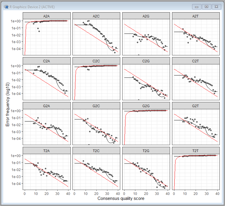
There are a total of 12 possible nucleotide transition (e.g., A→C, A→G, …). The plot shows the pair-wise transition of A, T, C and G (including self). The dots indicate the observed error rates for each consensus quality score. The black lines are the estimated error rates after convergence of the machine-learning algorithm. The red lines are the error rates expected under the nominal definition of the Q-score. Ideally we want to see a good fit between the black dots and the black line. As you can see the higher the quality scores the lower the error frequencies.
| This step is computationally intensive, we used the default setting for the learnErrors function and used only first 100M bases to learn error model. If you don't see a roughly good fit between dots and the lines, you can try increasing the "nbases" parameter to see if the fit improves. |
Step 6. De-replicate reads
Dereplication is to remove the redundant/repeated sequences from a set of sequences and keep only one copy of all the unique seuqences. Dereplication serves two purposes:
- Reduce computaton time by emiminating repeated sequences.
- The abudnace (copy number) infomration will be used in the partitioning step to form amplicon sequence variants.
Perform the following commands to dereplicate the reads:
#derepFastq.start=Sys.time()
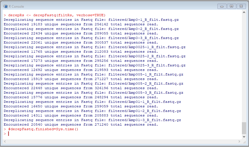
derepFs <- derepFastq(filtFs, verbose=TRUE)
derepRs <- derepFastq(filtRs, verbose=TRUE)
#derepFastq.finished=Sys.time()
The result should be self-explanatory:
 )
)
Step 7. Denoise sequences based on the error model to product amplicon sequence variants (ASVs)
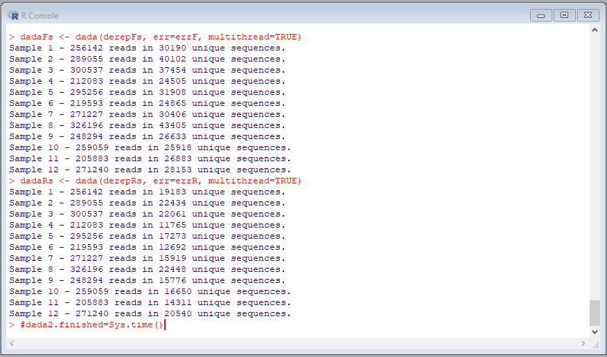
This step is the central part of the DADA2 pipeline. In a very simplified version of explanation, DADA2 uses a consensus quality profile with the abundance information to partition the reads into amplicaon sequence variants (ASVs). In a sample, if a sequence is real and abundant, there should be many identical copies of the same sequences. The more copies of the same sequences, the more likely it is to be true sequences. DADA2 partition the reads based on most abundant unique reads, and then forms ASVs using the consensus quality information associated with the reads.
Copy and paste the following R codes to perform the denoising step
names(derepFs) <- sample.names
names(derepRs) <- sample.names

#dada2.start=Sys.time()
dadaFs <- dada(derepFs, err=errF, multithread=TRUE)
dadaRs <- dada(derepRs, err=errR, multithread=TRUE)
#dada2.finished=Sys.time()
Step 8. Merge the pair-end reads to single reads
Next we merge the forward (R1) and reverse (R2) reads together to generate the full denoised sequences. This is done by aligning the denoised R1 reads with the reverse-complement of the corresponding R2 reads.
Perform the following command to merge the pair-end reads, and generate a liste of the merged ASV sequences.
mergers <- mergePairs(dadaFs, derepFs, dadaRs, derepRs, verbose=TRUE)
seqtab <- makeSequenceTable(mergers)
write.table(t(seqtab),file="seqtab.txt",sep="\t",quote=FALSE)

Step 9. Identify chimera and remove them
The PCR step prior to the sequencing often generates chimera - a hybrid artifial sequences dervied from two different parent sequeces. The ASVs may still have these hybrid sequences and should be removed. Chimeric sequences are identified if they can be exactly reconstructed by combining a left-segment and a right-segment from two more abundant “parent” sequences. It is easier and more accurate to identify chimera from the denoised ASVs than the noisy raw sequences.
#bimera.start=Sys.time()
seqtab.nochim <- removeBimeraDenovo(seqtab, method="consensus", multithread=TRUE, verbose=TRUE)
#bimera.finished=Sys.time()
write.table(t(seqtab.nochim),file="seqtab.nochim",sep="\t",quote=FALSE)
write_xlsx(data.frame(seqtab.nochim),"seqtab.nochim.xlsx")
modified R
#derepFs <- derepFastq(filtFs, verbose=TRUE)
#derepRs <- derepFastq(filtRs, verbose=TRUE)
load("errF.RData")
load("errR.RData")
names(derepFs) <- sample.names
names(derepRs) <- sample.names
load("dadaFs.RData")
load("dadaRs.RData")
load("mergers.RData")
load("seqtab.nochim.RData")

write.table(t(seqtab.nochim),file="seqtab.nochim",sep="\t",quote=FALSE)

write_xlsx(data.frame(seqtab.nochim),"seqtab.nochim.xlsx")
Step 10. Make a summary table for the above processes
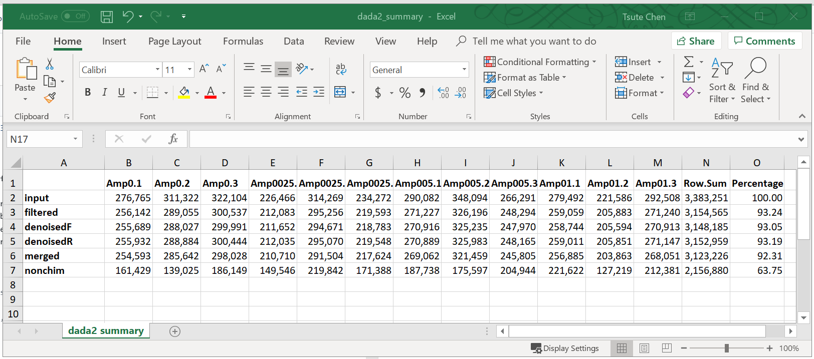
Use the following R codes to generate a summary of all the processes and keep track of number and percentage of reads after each step.
load("reads.filtered.RData")
getN <- function(x) sum(getUniques(x))
track <- cbind(reads.filtered, sapply(dadaFs, getN), sapply(dadaRs, getN), sapply(mergers, getN), rowSums(seqtab.nochim))
colnames(track) <- c("input", "filtered", "denoisedF", "denoisedR", "merged", "nonchim")
rownames(track) <- sample.names
track=rbind(track,colSums(track))
rownames(track)[nrow(track)]="Row Sum"
track=rbind(track,(track[nrow(track),]/track[nrow(track)])*100)
rownames(track)[nrow(track)]="Percentage"
write_xlsx(data.frame(t(track)),"dada2_summary.xlsx")
Step 11. Assign ASVs with taxonomy
The ASVs generated by DADA2 are the sequence variants and do not provide the taxonomy information. To find out which bacteria these ASVs may have come from, we need to compare these ASVS to a set of reference 16S rRNA sequences with taxonomy information. If an ASV is most similar to a reference sequence, the ASV can then be assigned to the taxonomy that is associated with the matching reference.
There are two general methods for finding the closest reference sequences (for the ASVs):
- Alignment: The closest reference sequence is identified based on highest sequence percent similarity calculated between aligned ASV and reference sequences.
- Non-alignment: the cloest reference sequence is identified based on the highest probability that the K-mers (e.g., all 8-mers in the ASVs) can be found in the reference.
The alignment based method provides percent similarity information thus once the cloest reference sequence is identified, we also know how close the ASV is to the reference, in term of percent sequence identity. This information is useful to determine whether the ASV is the same species (i.e., if 100% identical) of the reference. However the alignment is slow and can take a lot more computation time, especially if we are talking about millions of NGS reads. Luckily, the denoising process of DADA2 often reduces the number of reads from millions to hundreds, and thus drastically reduced the amount of time needed to calculate the percent similarity based on aligned sequences.
The K-mer based non-alignment method, on the other hand does not consider the position of the K-mer in the sequence and only calculate the (highest) possible probility for the vocabuary of K-mer words in an ASV to belong to a reference. Eventhough this method requires less computation time, the time diferennce between the alignment and non-alignment based methods is not significant when dealing with only hundreds of ASVs, rathaer than thousands of OTUs or millions of raw read data.
In this tutorial we will use the non-alignment taxonomy assignment method provided by the DADA2 package. This default k-mer based assignment is based on the naive Bayesian classifier method developed by the Ribosomal Database Project (RDP) (Wang et al, 2007. The fucntion is called “assignTaxonomy”.
The assignment will need a set of 16S rRNA gene reference sequences that is well curated with taxonomy information. There are several choices of the reference sequences. The DATA2 web site provides several choices:
- Silva version 132, Silva version 128, Silva version 123 (Silva dual-license)
- RDP trainset 16, RDP trainset 14
- GreenGenes version 13.8
- UNITE (use the General Fasta releases)
For this tutorial we will be using a set of reference sequences maintained by the HOMD project, this set of reference sequences includes:
- HMT RefSeq V15.1: 998sequences
- HOMD RefSeq Extended V1.11: 151 sequences
- GreenGeneGold V1: 2,623 sequences
- NCBI 16S rRNA Reference: 18,044sequences
- Mouse RefSeq V0.1: 82 sequences
All togethere there are 21,898 unique sequences representing a total of 14,651 prokarotic species. In addition the Genus names were added to the species level name so when the comparison is done at species level, the result will show the full scientific names for the species (i.e., Genus + Species).
This set of reference seuqences is included in the demo dataset in the taxonomy folder.
Copy and paste below R codes to perform the taxonomy assignement task:
#taxa.start=Sys.time()
taxa=assignTaxonomy(seqtab.nochim, "taxonomy/MOMDHOMDEXTGGNCBI_7S.fa.gz",tryRC=TRUE)
#taxa.finished=Sys.time()

taxa.print <- taxa
rownames(taxa.print) <- NULL
taxa.print
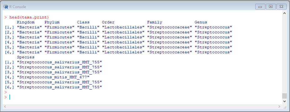
head(taxa.print)
Beginning of the taxa assignment output:
Once all the ASVs are all assgned with the potential taxonomy we are ready for many possible diversity analyses.